
Did you know that there’s one mistake…
…that thousands of data science beginners unknowingly commit?
And that this mistake can single-handedly ruin your machine learning model?
No, that’s not an exaggeration. We’re talking about one of the trickiest obstacles in applied machine learning: overfitting.
But don’t worry:
In this guide, we’ll walk you through exactly what overfitting means, how to spot it in your models, and what to do if your model is overfit.
By the end, you’ll know how to deal with this tricky problem once and for all.
Table of Contents
- Examples of Overfitting
- Signal vs. Noise
- Goodness of Fit
- Overfitting vs. Underfitting
- How to Detect Overfitting in Machine Learning
- How to Prevent Overfitting in Machine Learning
- Additional Resources
Examples of Overfitting
Let’s say we want to predict if a student will land a job interview based on her resume.
Now, assume we train a model from a dataset of 10,000 resumes and their outcomes.
Next, we try the model out on the original dataset, and it predicts outcomes with 99% accuracy… wow!
But now comes the bad news.
When we run the model on a new (“unseen”) dataset of resumes, we only get 50% accuracy… uh-oh!
Our model doesn’t generalize well from our training data to unseen data.
This is known as overfitting, and it’s a common problem in machine learning and data science.
In fact, overfitting occurs in the real world all the time. You only need to turn on the news channel to hear examples:
Signal vs. Noise
You may have heard of the famous book The Signal and the Noise by Nate Silver.
In predictive modeling, you can think of the “signal” as the true underlying pattern that you wish to learn from the data.
“Noise,” on the other hand, refers to the irrelevant information or randomness in a dataset.
For example, let’s say you’re modeling height vs. age in children. If you sample a large portion of the population, you’d find a pretty clear relationship:

This is the signal.
However, if you could only sample one local school, the relationship might be muddier. It would be affected by outliers (e.g. kid whose dad is an NBA player) and randomness (e.g. kids who hit puberty at different ages).
Noise interferes with signal.
Here’s where machine learning comes in. A well functioning ML algorithm will separate the signal from the noise.
If the algorithm is too complex or flexible (e.g. it has too many input features or it’s not properly regularized), it can end up “memorizing the noise” instead of finding the signal.
This overfit model will then make predictions based on that noise. It will perform unusually well on its training data… yet very poorly on new, unseen data.
Goodness of Fit
In statistics, goodness of fit refers to how closely a model’s predicted values match the observed (true) values.
A model that has learned the noise instead of the signal is considered “overfit” because it fits the training dataset but has poor fit with new datasets.

Overfitting vs. Underfitting
We can understand overfitting better by looking at the opposite problem, underfitting.
Underfitting occurs when a model is too simple – informed by too few features or regularized too much – which makes it inflexible in learning from the dataset.
Simple learners tend to have less variance in their predictions but more bias towards wrong outcomes (see: The Bias-Variance Tradeoff).
On the other hand, complex learners tend to have more variance in their predictions.
Both bias and variance are forms of prediction error in machine learning.
Typically, we can reduce error from bias but might increase error from variance as a result, or vice versa.
This trade-off between too simple (high bias) vs. too complex (high variance) is a key concept in statistics and machine learning, and one that affects all supervised learning algorithms.

How to Detect Overfitting in Machine Learning
A key challenge with overfitting, and with machine learning in general, is that we can’t know how well our model will perform on new data until we actually test it.
To address this, we can split our initial dataset into separate training and test subsets.

This method can approximate of how well our model will perform on new data.
If our model does much better on the training set than on the test set, then we’re likely overfitting.
For example, it would be a big red flag if our model saw 99% accuracy on the training set but only 55% accuracy on the test set.
If you’d like to see how this works in Python, we have a full tutorial for machine learning using Scikit-Learn.
Another tip is to start with a very simple model to serve as a benchmark.
Then, as you try more complex algorithms, you’ll have a reference point to see if the additional complexity is worth it.
This is the Occam’s razor test. If two models have comparable performance, then you should usually pick the simpler one.
How to Prevent Overfitting in Machine Learning
Detecting overfitting is useful, but it doesn’t solve the problem. Fortunately, you have several options to try.
Here are a few of the most popular solutions for overfitting:
Cross-validation
Cross-validation is a powerful preventative measure against overfitting.
The idea is clever: Use your initial training data to generate multiple mini train-test splits. Use these splits to tune your model.
In standard k-fold cross-validation, we partition the data into k subsets, called folds. Then, we iteratively train the algorithm on k-1 folds while using the remaining fold as the test set (called the “holdout fold”).

Cross-validation allows you to tune hyperparameters with only your original training set. This allows you to keep your test set as a truly unseen dataset for selecting your final model.
We have another article with a more detailed breakdown of cross-validation.
Train with more data
It won’t work every time, but training with more data can help algorithms detect the signal better. In the earlier example of modeling height vs. age in children, it’s clear how sampling more schools will help your model.
Of course, that’s not always the case. If we just add more noisy data, this technique won’t help. That’s why you should always ensure your data is clean and relevant.
Remove features
Some algorithms have built-in feature selection.
For those that don’t, you can manually improve their generalizability by removing irrelevant input features.
An interesting way to do so is to tell a story about how each feature fits into the model. This is like the data scientist’s spin on software engineer’s rubber duck debugging technique, where they debug their code by explaining it, line-by-line, to a rubber duck.
If anything doesn’t make sense, or if it’s hard to justify certain features, this is a good way to identify them.
In addition, there are several feature selection heuristics you can use for a good starting point.
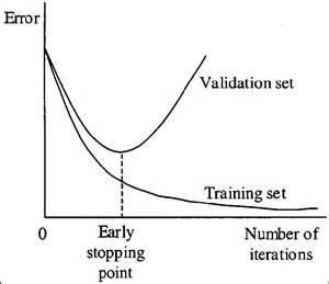
Early stopping
When you’re training a learning algorithm iteratively, you can measure how well each iteration of the model performs.
Up until a certain number of iterations, new iterations improve the model. After that point, however, the model’s ability to generalize can weaken as it begins to overfit the training data.
Early stopping refers stopping the training process before the learner passes that point.
Today, this technique is mostly used in deep learning while other techniques (e.g. regularization) are preferred for classical machine learning.
Regularization
Regularization refers to a broad range of techniques for artificially forcing your model to be simpler.
The method will depend on the type of learner you’re using. For example, you could prune a decision tree, use dropout on a neural network, or add a penalty parameter to the cost function in regression.
Oftentimes, the regularization method is a hyperparameter as well, which means it can be tuned through cross-validation.
We have a more detailed discussion here on algorithms and regularization methods.
Ensembling
Ensembles are machine learning methods for combining predictions from multiple separate models. There are a few different methods for ensembling, but the two most common are:
Bagging attempts to reduce the chance overfitting complex models.
- It trains a large number of “strong” learners in parallel.
- A strong learner is a model that’s relatively unconstrained.
- Bagging then combines all the strong learners together in order to “smooth out” their predictions.
Boosting attempts to improve the predictive flexibility of simple models.
- It trains a large number of “weak” learners in sequence.
- A weak learner is a constrained model (i.e. you could limit the max depth of each decision tree).
- Each one in the sequence focuses on learning from the mistakes of the one before it.
- Boosting then combines all the weak learners into a single strong learner.
While bagging and boosting are both ensemble methods, they approach the problem from opposite directions.
Bagging uses complex base models and tries to “smooth out” their predictions, while boosting uses simple base models and tries to “boost” their aggregate complexity.
Next Steps
Whew! We just covered quite a few concepts:
- Signal, noise, and how they relate to overfitting.
- Goodness of fit from statistics
- Underfitting vs. overfitting
- The bias-variance tradeoff
- How to detect overfitting using train-test splits
- How to prevent overfitting using cross-validation, feature selection, regularization, etc.
Hopefully seeing all of these concepts linked together helped clarify some of them.
To truly master this topic, we recommend getting hands-on practice.
While these concepts may feel overwhelming at first, they will ‘click into place’ once you start seeing them in the context of real-world code and problems.
So here are some additional resources to help you get started:
- Python machine learning tutorial
- Plotting overfitting and underfitting with Scikit-Learn
- More real-world examples of overfitting
Now, go forth and learn! (Or have your code do it for you!)